import subprocess, sys

def _pip_install(*pkgs):
    subprocess.run([sys.executable, "-m", "pip", "install", "-q", *pkgs], check=True)

_pip_install("pandas", "numpy", "matplotlib", "statsmodels")

import pathlib
import urllib.request

REPO = "MohammadYusif/time-series-forecasting-ai-systems"
BRANCH = "main"

def fetch(rel_path: str) -> str:
    """Locate rel_path from a repo checkout (tries rel_path and ../rel_path
    — labs live one directory below the repo root) or download it from
    GitHub if neither exists (a fresh Colab runtime)."""
    for candidate in (rel_path, f"../{rel_path}"):
        if pathlib.Path(candidate).exists():
            return candidate
    dest = pathlib.Path(pathlib.Path(rel_path).name)
    if not dest.exists():
        url = f"https://raw.githubusercontent.com/{REPO}/{BRANCH}/{rel_path}"
        urllib.request.urlretrieve(url, dest)
    return str(dest)

sys.path.insert(0, str(pathlib.Path(fetch("common/metrics.py")).parent))
from metrics import mae, rmse, mape, smape, wape, mase, pinball_loss, coverage, interval_width

sys.path.insert(0, str(pathlib.Path(fetch("common/backtest.py")).parent))
from backtest import seasonal_naive_forecast

import pandas as pd
import numpy as np
import matplotlib.pyplot as plt
%matplotlib inline

RNG_SEED = 20260912
np.random.seed(RNG_SEED)Lab 2 — Classical Forecasting: ARIMA & Exponential Smoothing

Lab 2 — Classical Forecasting: ARIMA & Exponential Smoothing
Hands-on companion to Classical Forecasting Models — objective 2 of this course. Using the same Riyadh/Grocery series and the same holdout convention as every lab in this course, we fit a SARIMAX chosen by a small AIC search, a Holt-Winters model, and a seasonal-naive baseline, forecast a 60-day holdout with each, and check the winning model’s residuals for leftover structure.
By the end you will have:
- run a real (small, bounded) order search over SARIMAX candidates and picked one by AIC,
- fit Holt-Winters and a seasonal-naive baseline on the exact same train/test split,
- scored all three with MAE/RMSE/WAPE/MASE from
common/metrics.py, and - run the Ljung-Box test on the winning model’s residuals and read what it does and doesn’t tell you.
Load and split — same convention as every lab in this course
Time-ordered holdout: the last 60 days are test, everything before is train. Never shuffle a time series before splitting it — a random split would let the model train on days that come after the days it’s being tested on, which is exactly the mistake day2/04_backtesting.qmd spends a whole lesson on. This lab’s single split is itself a simplification Lab 4 will revisit with several folds instead of one.
df = pd.read_csv(fetch("data/retail_demand.csv"), parse_dates=["date"])
riyadh_grocery = df[(df["region"] == "Riyadh") & (df["category"] == "Grocery")].copy()
riyadh_grocery = riyadh_grocery.set_index("date")["units_sold"].asfreq("D")

HORIZON = 60
train = riyadh_grocery.iloc[:-HORIZON]
test = riyadh_grocery.iloc[-HORIZON:]

print(f"train: {train.index.min().date()} .. {train.index.max().date()} ({len(train)} days)")
print(f"test:  {test.index.min().date()} .. {test.index.max().date()} ({len(test)} days)")

fig, ax = plt.subplots(figsize=(12, 4))
train.plot(ax=ax, linewidth=0.8, label="train")
test.plot(ax=ax, linewidth=0.8, label="test (holdout)")
ax.axvline(test.index[0], color="black", linestyle="--", linewidth=1, alpha=0.6)
ax.set_title("Riyadh / Grocery — 60-day holdout, no shuffling")
ax.legend()
plt.tight_layout()
plt.show()
train: 2023-01-01 .. 2025-11-01 (1036 days)
test: 2025-11-02 .. 2025-12-31 (60 days)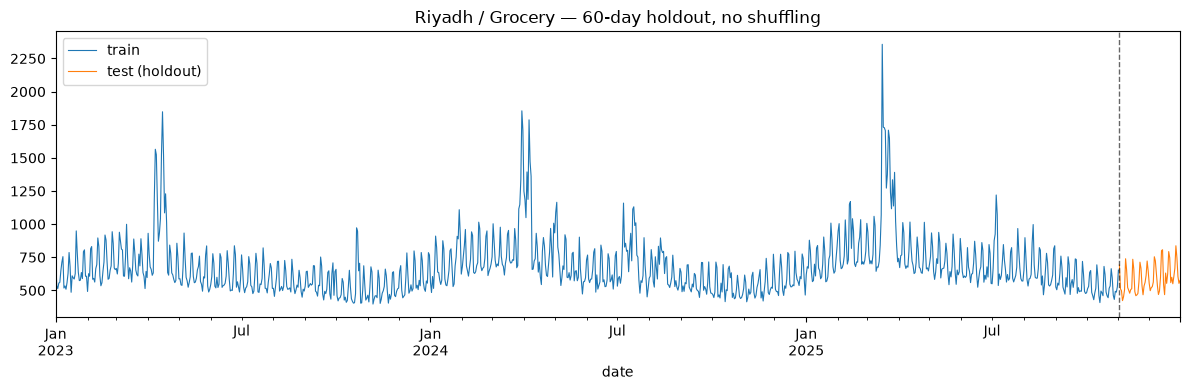
A small SARIMAX order search, selected by AIC
Lab 1’s ACF/PACF read suggested a short AR/MA order plus a seasonal term at s=7. Rather than guess one order, we search a small, bounded grid of candidates and let AIC — not intuition — pick the winner. This is a teaching-scale search (27 x 8 = 216 candidates, most converging in well under a second each); a production search would likely go wider, but the method — fit several, compare AIC, pick the minimum — is the same at any scale.
import itertools
import warnings

from statsmodels.tsa.statespace.sarimax import SARIMAX

warnings.filterwarnings("ignore")  # SARIMAX is chatty about convergence during a grid search

# A small, deliberately cheap grid — this is a teaching example of ORDER
# SELECTION BY AIC, not an exhaustive production search. Lab 1's ACF/PACF
# read pointed at a short AR/MA order plus a seasonal term at s=7; this
# grid brackets that read rather than searching blindly.
p_range = d_range = q_range = range(0, 3)
P_range = D_range = Q_range = range(0, 2)
SEASONAL_PERIOD = 7

results = []
for p, d, q in itertools.product(p_range, d_range, q_range):
    for P, D, Q in itertools.product(P_range, D_range, Q_range):
        try:
            model = SARIMAX(
                train,
                order=(p, d, q),
                seasonal_order=(P, D, Q, SEASONAL_PERIOD),
                enforce_stationarity=False,
                enforce_invertibility=False,
            )
            fit = model.fit(disp=False)
            results.append({"order": (p, d, q), "seasonal_order": (P, D, Q, SEASONAL_PERIOD), "aic": fit.aic})
        except Exception:
            continue  # a handful of orders fail to converge — skip, don't crash the search

results_df = pd.DataFrame(results).sort_values("aic").reset_index(drop=True)
print(f"{len(results_df)} / {len(list(itertools.product(p_range, d_range, q_range))) * len(list(itertools.product(P_range, D_range, Q_range)))} candidate orders converged")
print(results_df.head(8).to_string(index=False))

best = results_df.iloc[0]
print(f"\nBest by AIC: order={best['order']}, seasonal_order={best['seasonal_order']}, AIC={best['aic']:.2f}")
216 / 216 candidate orders converged
order seasonal_order aic
(1, 1, 2) (0, 1, 1, 7) 12264.838990
(1, 0, 2) (1, 1, 1, 7) 12269.368261
(2, 1, 1) (1, 1, 1, 7) 12270.124682
(2, 0, 2) (0, 1, 1, 7) 12271.494330
(2, 1, 2) (0, 1, 1, 7) 12272.032053
(1, 0, 2) (0, 1, 1, 7) 12274.515238
(2, 1, 1) (0, 1, 1, 7) 12275.330714
(2, 0, 1) (1, 1, 1, 7) 12278.471040
Best by AIC: order=(1, 1, 2), seasonal_order=(0, 1, 1, 7), AIC=12264.84Fit the winning SARIMAX and forecast the holdout
best_order = best["order"]
best_seasonal_order = best["seasonal_order"]

sarima_fit = SARIMAX(
    train,
    order=best_order,
    seasonal_order=best_seasonal_order,
    enforce_stationarity=False,
    enforce_invertibility=False,
).fit(disp=False)

print(sarima_fit.summary().tables[0])

sarima_forecast = sarima_fit.get_forecast(steps=HORIZON).predicted_mean
sarima_forecast.index = test.index
SARIMAX Results
===========================================================================================
Dep. Variable: units_sold No. Observations: 1036
Model: SARIMAX(1, 1, 2)x(0, 1, [1], 7) Log Likelihood -6127.419
Date: Sat, 12 Sep 2026 AIC 12264.839
Time: 19:34:21 BIC 12289.467
Sample: 01-01-2023 HQIC 12274.191
- 11-01-2025
Covariance Type: opg
===========================================================================================Holt-Winters (additive trend, additive seasonality)
from statsmodels.tsa.holtwinters import ExponentialSmoothing

hw_fit = ExponentialSmoothing(
    train, trend="add", seasonal="add", seasonal_periods=SEASONAL_PERIOD
).fit()

hw_forecast = hw_fit.forecast(HORIZON)
hw_forecast.index = test.index

alpha = hw_fit.params["smoothing_level"]
beta = hw_fit.params["smoothing_trend"]
gamma = hw_fit.params["smoothing_seasonal"]
print(f"Holt-Winters: alpha={alpha:.4f}, beta={beta:.4f}, gamma={gamma:.4f}")
Holt-Winters: alpha=0.7326, beta=0.0000, gamma=0.0000The baseline every model here has to beat
seasonal_naive_forecast from common/backtest.py simply repeats the last observed 7-day cycle forward. It costs nothing to compute and has no parameters to get wrong — which is exactly why it’s the right floor to compare against.
naive_forecast_values = seasonal_naive_forecast(train.to_numpy(), horizon=HORIZON, period=SEASONAL_PERIOD)
naive_forecast = pd.Series(naive_forecast_values, index=test.index)
All three forecasts against the actual holdout
fig, ax = plt.subplots(figsize=(13, 5))
train.iloc[-90:].plot(ax=ax, linewidth=0.8, color="black", label="train (last 90 days)")
test.plot(ax=ax, linewidth=1.2, color="black", linestyle=":", label="actual (holdout)")
sarima_forecast.plot(ax=ax, linewidth=1.2, label=f"SARIMAX{best_order}x{best_seasonal_order}")
hw_forecast.plot(ax=ax, linewidth=1.2, label="Holt-Winters")
naive_forecast.plot(ax=ax, linewidth=1.2, label="seasonal-naive")
ax.axvline(test.index[0], color="gray", linestyle="--", linewidth=1)
ax.set_title("60-day holdout — SARIMAX vs Holt-Winters vs seasonal-naive")
ax.legend()
plt.tight_layout()
plt.show()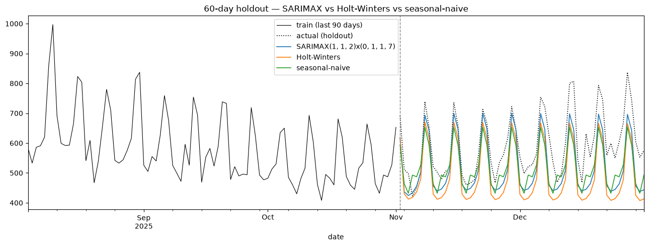
Scoring
mase is scaled against the seasonal-naive baseline computed on train itself (seasonal_period=7) — a value below 1.0 means a model beat that baseline; above 1.0 means it did worse than just repeating last week.
y_true = test.to_numpy()
y_train_arr = train.to_numpy()

rows = []
for name, y_pred in [
    ("SARIMAX", sarima_forecast.to_numpy()),
    ("Holt-Winters", hw_forecast.to_numpy()),
    ("seasonal-naive", naive_forecast.to_numpy()),
]:
    rows.append({
        "model": name,
        "mae": mae(y_true, y_pred),
        "rmse": rmse(y_true, y_pred),
        "wape": wape(y_true, y_pred),
        "mase": mase(y_true, y_pred, y_train_arr, seasonal_period=SEASONAL_PERIOD),
    })

scores = pd.DataFrame(rows).set_index("model").sort_values("mase")
scores.style.format("{:.3f}")| mae | rmse | wape | mase | |
|---|---|---|---|---|
| model | ||||
| SARIMAX | 71.190 | 86.263 | 12.053 | 0.785 |
| seasonal-naive | 78.133 | 91.609 | 13.228 | 0.862 |
| Holt-Winters | 99.745 | 111.925 | 16.887 | 1.100 |
Residual diagnostics — Ljung-Box
A well-fit model’s residuals should look like noise: no leftover autocorrelation for the model to have captured but didn’t. Ljung-Box tests exactly that, at a chosen set of lags. Its null hypothesis is “the residuals are independently distributed” (i.e. no leftover autocorrelation) — so, reading the direction the same way Lab 1’s ADF discussion did: a low p-value here is the bad outcome (reject the null → structure remains that the model missed), and a high p-value is what you want (residuals look like noise).
from statsmodels.stats.diagnostic import acorr_ljungbox

lb = acorr_ljungbox(sarima_fit.resid, lags=[7, 14, 21], return_df=True)
print(lb)

fig, ax = plt.subplots(figsize=(12, 3))
sarima_fit.resid.plot(ax=ax, linewidth=0.6)
ax.axhline(0, color="black", linewidth=0.5)
ax.set_title(f"SARIMAX{best_order}x{best_seasonal_order} residuals")
plt.tight_layout()
plt.show()
lb_stat lb_pvalue
7 12.039669 0.099262
14 31.101940 0.005364
21 36.207577 0.020720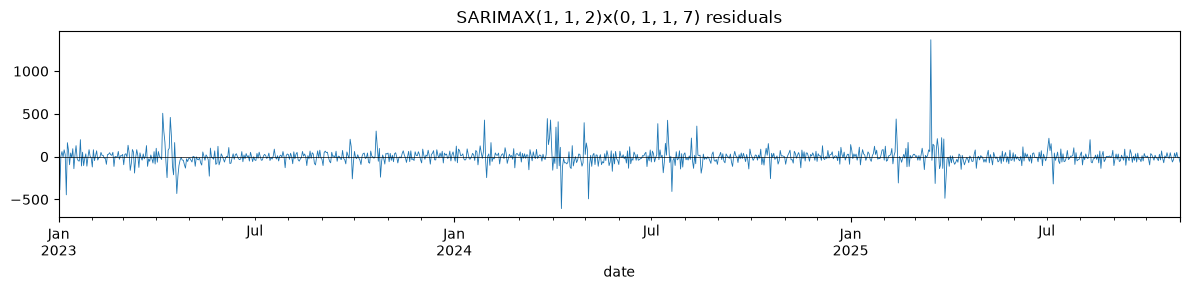
What actually happened
Order selected by AIC: SARIMAX
(1, 1, 2)x(0, 1, 1, 7)— the best of all 216/216 candidate orders in the grid that converged.Holt-Winters degenerated on this series: the fitted smoothing parameters came back
alpha=0.7326, beta=0.0000, gamma=0.0000— the optimizer set both the trend and seasonal smoothing weights to zero, meaning the model effectively fell back to simple exponential smoothing with no real trend or seasonal component, despite being asked for both. This is a genuine, worth-noticing result, not a bug in the lab: additive Holt-Winters assumes seasonal swings of roughly constant absolute size, and this series’ weekly swing grows with its level exactly the wayday2/03_feature_engineering.qmd’s multiplicative-generator discussion describes — a model built for additive seasonality has a genuine reason to struggle here.Scores on the 60-day holdout (lower is better; MASE below 1.0 beats the seasonal-naive baseline it’s scaled against):
model mae rmse wape mase SARIMAX 71.190 86.263 12.053 0.785 seasonal-naive 78.133 91.609 13.228 0.862 Holt-Winters 99.745 111.925 16.887 1.100 SARIMAX wins, and Holt-Winters actually loses to the naive baseline on this holdout — not the tidy “every classical method beats naive” story a lesson might be tempted to tell, but the real result. It’s a direct consequence of the degenerate fit above: a Holt-Winters model that isn’t actually using its trend/seasonal terms has no real advantage left over seasonal-naive, and the small amount of daily noise put it slightly behind it on this particular 60-day window. (
day3/06_lab_model_comparison.ipynbrefits Holt-Winters fresh across 12 different, larger training windows on this same series and finds it winning there instead — a concrete illustration that a single split’s verdict on a model family can be an artifact of exactly where that split happened to fall, not a stable property of the model. That is the whole reasonday2/04_backtesting.qmdinsists on more than one holdout.)Ljung-Box on the SARIMAX residuals: p=0.099 at lag 7, but p=0.005 at lag 14 and p=0.021 at lag 21 — both comfortably below 0.05. Reading the direction correctly (low p-value → reject the “residuals are independent” null → structure remains): this model has not fully whitened its residuals at the longer lags. Some autocorrelation the order search didn’t capture is still there at 2-3 week horizons — plausibly related to the drifting holiday-style bumps
01_lab_decomposition.ipynbfound sitting in the STL residual, which a fixed(P,D,Q)_7seasonal term has no way to represent.
Closing thoughts
The headline result here — SARIMAX beats a naive baseline that itself beats Holt-Winters — is a single 60-day draw. day2/04_lab_backtesting_framework.ipynb checks whether this exact ranking survives being tested across several holdouts instead of one, which is precisely the question a single split like this one cannot answer on its own.
One honest limitation of everything on this page: the SARIMA order search above only compares AIC across combinations of (p,d,q) and (P,D,Q) at a fixed seasonal period. It never questions whether s=7 itself was the right seasonal period to search over in the first place — Lab 1’s ACF/PACF read is what justified that choice, not this cell. And the Ljung-Box result above is a reason to want more than an AIC-selected order in practice — a real project would likely also try adding exogenous regressors for the holiday-style bumps rather than asking a bigger (P,D,Q)_7 term to absorb them.
Continue to Day 2: Feature Engineering for Tree-Based Forecasting