import subprocess, sys

def _pip_install(*pkgs):
    subprocess.run([sys.executable, "-m", "pip", "install", "-q", *pkgs], check=True)

_pip_install("pandas", "numpy", "matplotlib", "scikit-learn", "lightgbm", "statsmodels")

import pathlib
import urllib.request

REPO = "MohammadYusif/time-series-forecasting-ai-systems"
BRANCH = "main"

def fetch(rel_path: str) -> str:
    """Locate rel_path from a repo checkout (tries rel_path and ../rel_path
    — labs live one directory below the repo root) or download it from
    GitHub if neither exists (a fresh Colab runtime)."""
    for candidate in (rel_path, f"../{rel_path}"):
        if pathlib.Path(candidate).exists():
            return candidate
    dest = pathlib.Path(pathlib.Path(rel_path).name)
    if not dest.exists():
        url = f"https://raw.githubusercontent.com/{REPO}/{BRANCH}/{rel_path}"
        urllib.request.urlretrieve(url, dest)
    return str(dest)

sys.path.insert(0, str(pathlib.Path(fetch("common/metrics.py")).parent))
from metrics import mae, rmse, mape, smape, wape, mase, pinball_loss, coverage, interval_width
sys.path.insert(0, str(pathlib.Path(fetch("common/backtest.py")).parent))
from backtest import expanding_window_splits, rolling_window_splits, run_backtest, seasonal_naive_forecast

import pandas as pd
import numpy as np
import matplotlib.pyplot as plt
%matplotlib inline

RNG_SEED = 20260912
np.random.seed(RNG_SEED)Lab 4 — Does the Verdict Survive More Than One Holdout?

Lab 4 — Does the verdict survive more than one holdout?
Labs 2 and 3 each picked apart one model’s fit on this same Riyadh / Grocery series using a single held-out window — one fixed slice of time, one number per model, one ranking. That’s enough to notice a model is roughly competitive, but it hides a real risk: a 60-day window can be a run of unusually calm (or unusually chaotic) weeks by chance, and the model that wins on that one window is not necessarily the model that wins in general.
This lab builds the walk-forward harness objective 4 is about: instead of one train/test split, common/backtest.py’s expanding_window_splits carves out 5 folds, each a 14-day test window, each trained on everything before it (an expanding window — fold 4’s training set is strictly larger than fold 0’s, because by fold 4 more real history has actually happened). We run the same three model families — seasonal-naive, Holt-Winters, and a recursive LightGBM — through all 5 folds and look at the spread across folds, not just the average, because the spread is exactly the information a single train/test split throws away.
Load the data
Same Riyadh / Grocery series Labs 2 and 3 used.
df = pd.read_csv(fetch("data/retail_demand.csv"), parse_dates=["date"])
series_df = (
    df[(df["region"] == "Riyadh") & (df["category"] == "Grocery")]
    .set_index("date")
    .asfreq("D")
    .sort_index()
)
series = series_df["units_sold"]
print(f"{len(series)} daily observations, {series.index.min().date()} to {series.index.max().date()}")
print(f"missing values after asfreq: {series.isna().sum()}")
series.plot(figsize=(11, 3), title="Riyadh / Grocery — daily units sold")
plt.tight_layout()
1096 daily observations, 2023-01-01 to 2025-12-31
missing values after asfreq: 0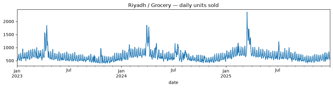
Build the walk-forward splits
n_folds=5, horizon=14, min_train_size=730 — every fold trains on at least ~2 years of history and is tested on the 14 days right after it, and the last fold’s test window ends on the series’ final real day.
N_FOLDS = 5
HORIZON = 14
MIN_TRAIN_SIZE = 730  # ~2 years minimum history before the first fold

splits = expanding_window_splits(
    n=len(series), n_folds=N_FOLDS, horizon=HORIZON, min_train_size=MIN_TRAIN_SIZE
)

SERIES_START = series.index[0]  # every fold's train slice starts at position 0

for i, (train_slice, test_slice) in enumerate(splits):
    train_start_date = SERIES_START
    train_end_date = series.index[train_slice.stop - 1]
    test_start_date = series.index[test_slice.start]
    test_end_date = series.index[test_slice.stop - 1]
    print(
        f"fold {i}: train {train_start_date.date()} -> {train_end_date.date()} "
        f"({train_slice.stop} days)  |  test {test_start_date.date()} -> {test_end_date.date()}"
    )
fold 0: train 2023-01-01 -> 2025-10-22 (1026 days) | test 2025-10-23 -> 2025-11-05
fold 1: train 2023-01-01 -> 2025-11-05 (1040 days) | test 2025-11-06 -> 2025-11-19
fold 2: train 2023-01-01 -> 2025-11-19 (1054 days) | test 2025-11-20 -> 2025-12-03
fold 3: train 2023-01-01 -> 2025-12-03 (1068 days) | test 2025-12-04 -> 2025-12-17
fold 4: train 2023-01-01 -> 2025-12-17 (1082 days) | test 2025-12-18 -> 2025-12-31Three models, one interface
Each model is wrapped as a fit_predict_fn(y_train, horizon) — run_backtest calls it fresh for every fold, so refitting per fold is automatic, not something we have to remember to do.
Seasonal-naive — the floor
def naive_fit_predict(y_train, horizon):
    """The floor every model here is expected to beat: repeat the last
    observed weekly cycle. No fitting at all — same call signature as the
    other two so it can go through the exact same `run_backtest` loop."""
    return seasonal_naive_forecast(y_train, horizon, period=7)


naive_results = run_backtest(series.values, splits, naive_fit_predict)
print(f"ran {len(naive_results)} folds for seasonal-naive")
ran 5 folds for seasonal-naiveHolt-Winters (ExponentialSmoothing)
from statsmodels.tsa.holtwinters import ExponentialSmoothing
import warnings


def holt_winters_fit_predict(y_train, horizon):
    """Fit a fresh Holt-Winters model on exactly this fold's y_train and
    forecast `horizon` steps ahead. Refitting inside the callable (rather
    than fitting once outside the fold loop) is what makes this a fair
    walk-forward comparison: fold 0 never sees a model that was also
    calibrated on fold 3's or fold 4's data."""
    with warnings.catch_warnings():
        warnings.simplefilter("ignore")
        model = ExponentialSmoothing(
            y_train, trend="add", seasonal="add", seasonal_periods=7
        ).fit()
    return model.forecast(horizon)


hw_results = run_backtest(series.values, splits, holt_winters_fit_predict)
print(f"ran {len(hw_results)} folds for Holt-Winters")
ran 5 folds for Holt-WintersLightGBM: features + recursive multi-step forecasting
LightGBM has no notion of time — it needs the same kind of lag/rolling/ calendar features Day 2’s feature-engineering lesson introduces. The feature function below mirrors that lesson: lagged values, rolling statistics computed only from past observations, and calendar fields.
Because run_backtest hands fit_predict_fn a plain y_train array (not a dated Series), and expanding_window_splits always starts every fold’s train slice at position 0, fold i‘s y_train always begins on the series’ actual first date (SERIES_START, captured above). That lets us reconstruct a real DatetimeIndex for y_train inside the callable — pd.date_range(start=SERIES_START, periods=len(y_train), freq="D") — and get real calendar features without ever needing to pass dates through run_backtest itself.
Forecasting 14 steps ahead recursively means step 2’s lag_1 feature is step 1’s prediction, not a true future value that hasn’t happened yet in this fold. The loop below does that explicitly: each step appends its own prediction to a working history before computing the next step’s features.
FEATURE_COLS = [
    "lag_1", "lag_7", "lag_14", "lag_28",
    "roll_mean_7", "roll_mean_28", "roll_std_7",
    "dow", "is_weekend", "day", "month",
]


def make_features(y: pd.Series) -> pd.DataFrame:
    """Lag, rolling-window, and calendar features for a dated Series `y`.
    Every rolling/lag feature is built from `y.shift(1)` onward, so the
    feature for date t never touches y[t] itself — only strictly earlier
    values."""
    feat = pd.DataFrame({"y": y})
    feat["lag_1"] = y.shift(1)
    feat["lag_7"] = y.shift(7)
    feat["lag_14"] = y.shift(14)
    feat["lag_28"] = y.shift(28)
    shifted = y.shift(1)
    feat["roll_mean_7"] = shifted.rolling(7).mean()
    feat["roll_mean_28"] = shifted.rolling(28).mean()
    feat["roll_std_7"] = shifted.rolling(7).std()
    feat["dow"] = feat.index.dayofweek
    feat["is_weekend"] = (feat.index.dayofweek >= 5).astype(int)
    feat["day"] = feat.index.day
    feat["month"] = feat.index.month
    return feat
import lightgbm as lgb
def lightgbm_recursive_fit_predict(y_train, horizon):
"""Fit fresh on this fold's y_train only, then forecast recursively:
predict step 1, append it to the working history, recompute features
(now including that prediction as the newest lag_1), predict step 2,
and so on. `make_features` is called fresh here on THIS fold's
reconstructed history — never on the full series computed once outside
the fold loop — so a model trained on fold 0 has literally never seen
a feature value derived from 2025 data."""
idx = pd.date_range(start=SERIES_START, periods=len(y_train), freq="D")
history = pd.Series(y_train, index=idx)
train_feat = make_features(history).dropna()
model = lgb.LGBMRegressor(
n_estimators=200,
num_leaves=15,
learning_rate=0.05,
min_child_samples=10,
verbosity=-1,
)
model.fit(train_feat[FEATURE_COLS], train_feat["y"])
working = history.copy()
preds = []
for _ in range(horizon):
next_date = working.index[-1] + pd.Timedelta(days=1)
extended = pd.concat([working, pd.Series([np.nan], index=[next_date])])
next_feat = make_features(extended).loc[[next_date], FEATURE_COLS]
pred = float(model.predict(next_feat)[0])
preds.append(pred)
# the prediction becomes part of the working history that feeds
# the NEXT step's lag/rolling features — this is what makes the
# forecast recursive instead of leaking true future values.
working.loc[next_date] = pred
return np.array(preds)
lgb_results = run_backtest(series.values, splits, lightgbm_recursive_fit_predict)
print(f"ran {len(lgb_results)} folds for LightGBM (recursive)")ran 5 folds for LightGBM (recursive)Score every fold
mae in raw units, wape as a scale-free percentage, and mase scaled against that fold’s own seasonal-naive in-sample error (seasonal_period=7) — a fold with an unusually calm or volatile training window gets its own yardstick, not one borrowed from a different fold.
MODEL_RESULTS = {
    "seasonal_naive": naive_results,
    "holt_winters": hw_results,
    "lightgbm_recursive": lgb_results,
}

rows = []
for model_name, fold_results in MODEL_RESULTS.items():
    for r in fold_results:
        rows.append({
            "fold": r["fold"],
            "model": model_name,
            "mae": mae(r["y_true"], r["y_pred"]),
            "wape": wape(r["y_true"], r["y_pred"]),
            "mase": mase(r["y_true"], r["y_pred"], r["y_train"], seasonal_period=7),
        })

results_df = pd.DataFrame(rows).sort_values(["model", "fold"]).reset_index(drop=True)
results_df| fold | model | mae | wape | mase | |
|---|---|---|---|---|---|
| 0 | 0 | holt_winters | 34.305928 | 6.414036 | 0.375902 |
| 1 | 1 | holt_winters | 30.124846 | 5.488650 | 0.332556 |
| 2 | 2 | holt_winters | 37.943274 | 6.579215 | 0.422691 |
| 3 | 3 | holt_winters | 40.484061 | 6.633624 | 0.454839 |
| 4 | 4 | holt_winters | 30.590591 | 4.751673 | 0.345060 |
| 5 | 0 | lightgbm_recursive | 28.827452 | 5.389748 | 0.315872 |
| 6 | 1 | lightgbm_recursive | 28.433259 | 5.180448 | 0.313883 |
| 7 | 2 | lightgbm_recursive | 35.608106 | 6.174306 | 0.396677 |
| 8 | 3 | lightgbm_recursive | 48.702156 | 7.980222 | 0.547169 |
| 9 | 4 | lightgbm_recursive | 45.172030 | 7.016625 | 0.509537 |
| 10 | 0 | seasonal_naive | 36.142857 | 6.757479 | 0.396030 |
| 11 | 1 | seasonal_naive | 35.714286 | 6.507028 | 0.394260 |
| 12 | 2 | seasonal_naive | 40.285714 | 6.985385 | 0.448786 |
| 13 | 3 | seasonal_naive | 58.714286 | 9.620787 | 0.659655 |
| 14 | 4 | seasonal_naive | 61.214286 | 9.508488 | 0.690493 |
Mean and standard deviation per model, across the 5 folds:
summary = results_df.groupby("model")[["mae", "wape", "mase"]].agg(["mean", "std"])
summary| mae | wape | mase | ||||
|---|---|---|---|---|---|---|
| mean | std | mean | std | mean | std | |
| model | ||||||
| holt_winters | 34.689740 | 4.526263 | 5.973440 | 0.825328 | 0.386209 | 0.051766 |
| lightgbm_recursive | 37.348601 | 9.290208 | 6.348270 | 1.164346 | 0.416628 | 0.108143 |
| seasonal_naive | 46.414286 | 12.528783 | 7.875833 | 1.551424 | 0.517845 | 0.145601 |
The spread, not just the mean
This is the plot a single train/test split can never produce: the same model’s score across 5 different, non-overlapping test windows.
fig, axes = plt.subplots(1, 2, figsize=(12, 4.5))

models = list(MODEL_RESULTS.keys())
wape_by_model = [results_df.loc[results_df["model"] == m, "wape"].values for m in models]
mase_by_model = [results_df.loc[results_df["model"] == m, "mase"].values for m in models]

axes[0].boxplot(wape_by_model, tick_labels=models)
axes[0].set_ylabel("WAPE (%)")
axes[0].set_title("WAPE spread across 5 folds")
axes[0].tick_params(axis="x", rotation=20)

axes[1].boxplot(mase_by_model, tick_labels=models)
axes[1].axhline(1.0, color="gray", linestyle="--", linewidth=1, label="naive baseline (MASE=1)")
axes[1].set_ylabel("MASE")
axes[1].set_title("MASE spread across 5 folds")
axes[1].tick_params(axis="x", rotation=20)
axes[1].legend(fontsize=8)

plt.tight_layout()
plt.show()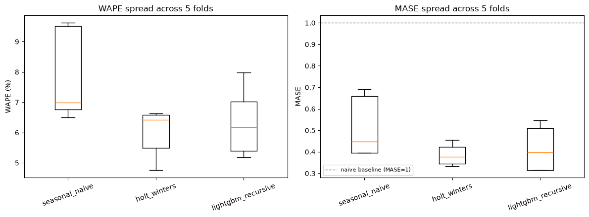
Discussion — did the ranking hold up?
One part of the ranking is completely stable: seasonal-naive is the worst model in every single fold (WAPE 6.76, 6.51, 6.99, 9.62, 9.51 — never close to either real model). That part of Lab 2/3’s verdict would have held up no matter which 60-day window got picked.
The Holt-Winters vs. LightGBM ordering is a different story — it flips:
| fold | Holt-Winters WAPE | LightGBM WAPE | winner |
|---|---|---|---|
| 0 | 6.41 | 5.39 | LightGBM |
| 1 | 5.49 | 5.18 | LightGBM |
| 2 | 6.58 | 6.17 | LightGBM |
| 3 | 6.63 | 7.98 | Holt-Winters |
| 4 | 4.75 | 7.02 | Holt-Winters |
LightGBM wins the first three folds (earlier, calmer test windows) and Holt-Winters wins the last two — including a decisive win in fold 4, the most recent 14 days in the series. If Lab 2 or Lab 3’s single 60-day-style holdout happened to land on that recent window, it would have reported Holt-Winters as the clear winner and LightGBM as clearly worse. Judged across all 5 folds instead, that verdict does not fully hold up: LightGBM actually wins a majority of folds (3 of 5), even though Holt-Winters ends up with the better mean WAPE (5.97 vs. 6.35) because its two wins are by a wider margin than its two losses. LightGBM also has almost 50% more fold-to-fold spread (WAPE std 1.16 vs. 0.83), which is exactly why a single holdout is a noisier estimate of its performance specifically.
The practical takeaway: a single 60-day-style holdout is a noisy estimate of one fold, not a reliable estimate of a model’s general performance — a real submission’s single-holdout ranking flipped when checked against 4 more folds here. Reporting the mean and the spread (or, better, showing every fold like the boxplots above) is what lets you tell “this model is reliably better” apart from “this model happened to win the window I picked.”
A concrete leakage check
The recursive LightGBM callable calls make_features on history = pd.Series(y_train, index=idx) — a Series built fresh inside lightgbm_recursive_fit_predict, from that fold’s own y_train only, every time run_backtest invokes it for a new fold. The line that actually keeps this sound is:
train_feat = make_features(history).dropna()This runs once per fold call, on that fold’s y_train alone — fold 0’s train_feat is built from history that only ever contains 2023’s early days, because y_train itself only ever contains those days. model = lgb.LGBMRegressor(...) is likewise instantiated and .fit() inside the same callable, so fold 0’s trained model has literally never seen a single row derived from 2025.
Contrast that with a version that would leak: if make_features had instead been called once, outside the fold loop, on the full series — e.g. ALL_FEATURES = make_features(series) computed before splits is even built, then sliced per fold afterward — the individual lag/rolling values would still be correct (they only look backward from each row), but anything stateful fit the same way would not be: a StandardScaler or target encoder fit once on series before the fold loop would hand fold 0’s training rows a mean and standard deviation computed using 2025 data that, from fold 0’s point of view, has not happened yet. This lab has no such scaler, but it is the same principle: everything that learns anything from data — the LightGBM model, and make_features’s own call site — is invoked fresh, inside the callable, once per fold.
Continue to the next lesson: Probabilistic Forecasting: Intervals, Quantiles, and Calibration